Stateball: a matchup-aware Monte Carlo on top of win expectancy

Baseball is a discrete game wrapped around a chaotic core. One batter, one pitcher, a finite state board, a century of recorded transitions, ten years of every pitch tracked. Win expectancy tables are the natural distillation: collapse the game to (inning, outs, bases, run diff), look up the historical home-win rate, and you get the number sitting on every live game card in my schedule view.

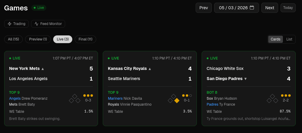
The table doesn't see the matchup. Every batter-pitcher pair in a given state averages into one number. What follows is the build that tries to put them back: a pitch-grain warehouse, a plate-appearance model, a sim that stitches them into games, and what came out the other end.

A half-inning has 24 states: 8 baserunner configurations across 3 out counts. Every plate appearance is a transition between two of those states, or the third out that ends the half and resets the board. An inning is a tree of transitions for each side; a game is nine of those, with the score and the pitcher state riding alongside.

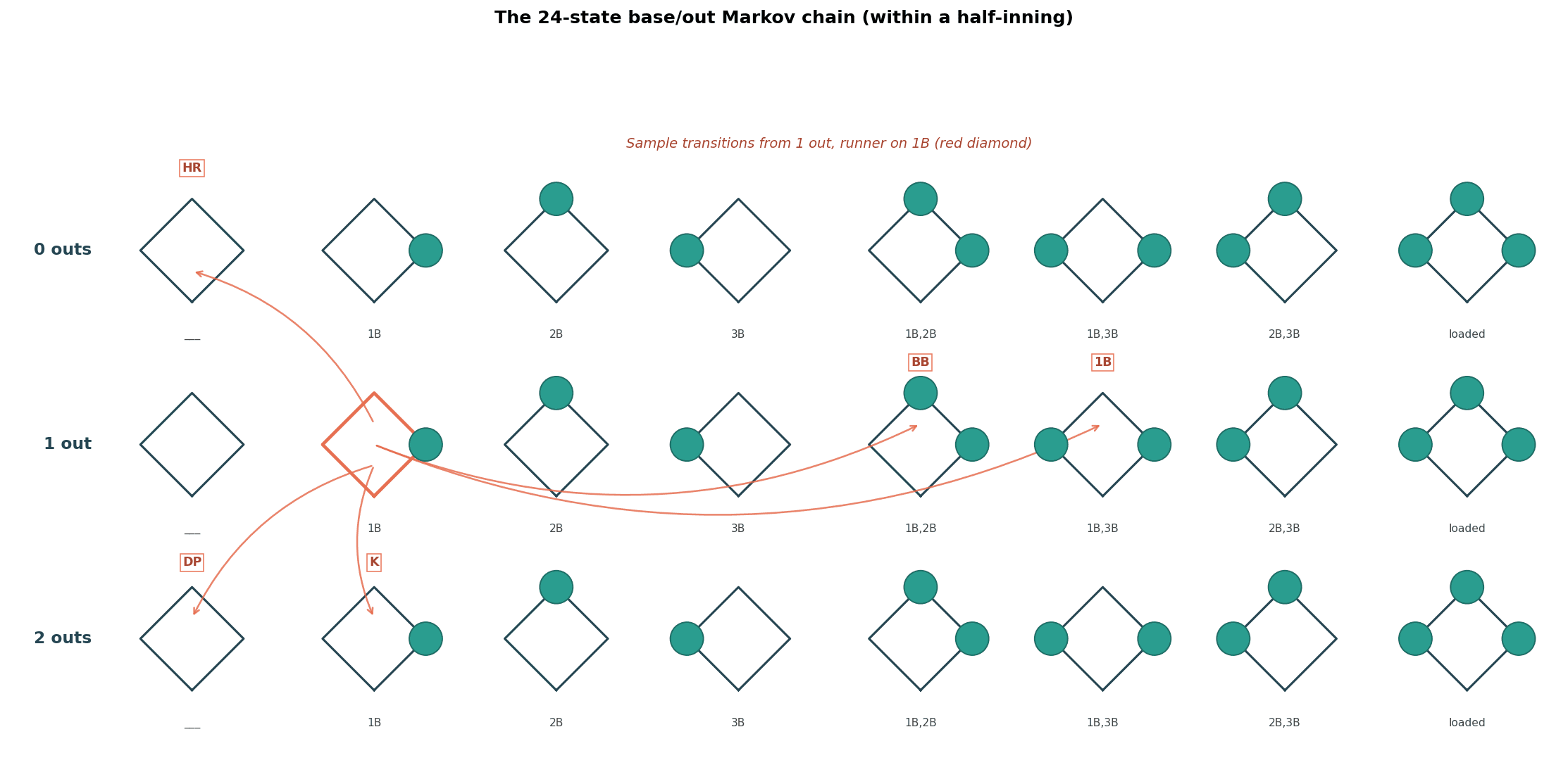
That's the inner loop. What sits on top is everything that makes one PA different from another: which batter, which pitcher, how the pitcher has been working tonight, which platoon split applies, who is on the bench. The discrete state board is the easy part. The transition probabilities are the hard part. They're not constants, they're a function of the matchup at that PA.

None of the framing here is new. George Lindsey (1963, Operations Research) first formalized the 24-state board and computed run expectancies from major-league play-by-play. Bukiet, Harold, and Palacios (1997) extended it into an explicit Markov-chain treatment for run distributions and game outcomes. Tango, Lichtman, and Dolphin's The Book (2007) standardized the run-expectancy and win-expectancy tables that the public-facing WE numbers descend from.

WE tables answer “what fraction of games has the home team won from this state, historically?” The sim answers “given who is about to come up against who is currently throwing, what does the rest of this game look like?” Same board, different transition function.

A couple of pieces ride along that I'm not going to dwell on: a baserunning sub-model (when does a runner go first-to-third on a single, when does the catcher's throw retire him), and a pitcher-exit model that handles the bullpen. Both feed into the same PA-level transitions.

Pitch-level data is the unit. Not plate appearance. Not at-bat. Pitch. Every Statcast pitch since 2015 has its release point, velocity, spin, location, and what happened. That granularity matters because the matchup conditioning the sim wants is built from how batters and pitchers actually behave at the pitch level: chase rates, whiff rates by zone, exit velocity on contact.

Even before you condition on the matchup, the count is doing most of the work. Baseball Bits' The Only Thing That Matters in Baseball puts a number on it: the worst hitters in baseball at 3-1 outperform the best hitters down 0-2. Same hitter, two different planets, depending on the count alone. The count state only exists if you're tracking every pitch.

The warehouse is DuckDB + DuckLake (Postgres metadata, S3 storage), dbt for transforms, Dagster for orchestration. The dbt project takes raw event data and walks it through intermediate models that resolve player references, build pitcher arsenals, compute batter platoon profiles, and finally assemble the feature vectors the model trains on.

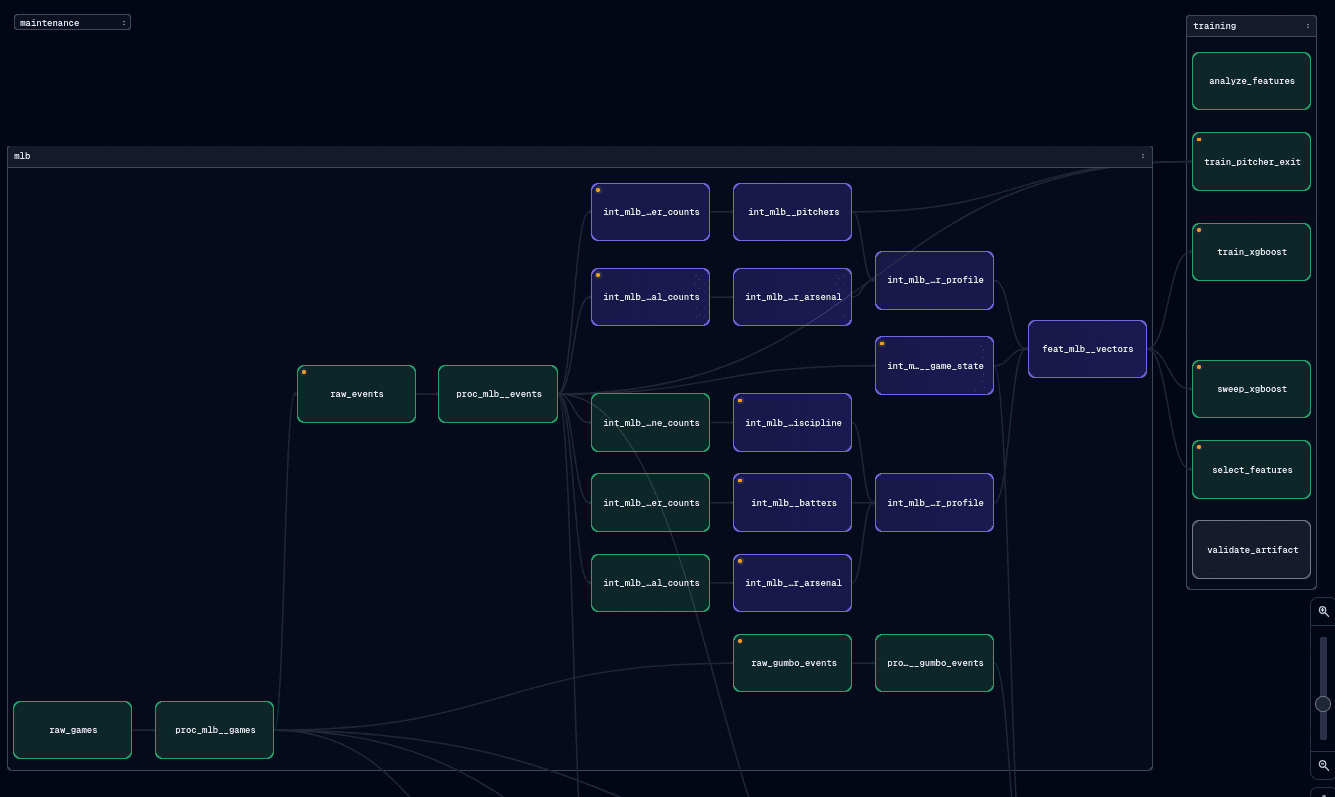
The asset graph has one job: turn ten years of pitch records into ~150 static features per batter-pitcher matchup, plus ~22 dynamic features per PA (count, score, base-out state, pitcher pitch count). The static features split by handedness (L/R batter against L/R pitcher, switch hitters resolved to the pitcher's opposite hand) and by horizon (season-to-date and career-to-date), all maintained at daily grain so that for any game on any date the features reflect only data through that day. No leakage from later games into earlier ones. Static features are pre-computed and cached; dynamic features fill in at sim time.

The same warehouse exposes the data as a queryable product: every player's season splits behind a stats view that mirrors what FanGraphs or Baseball Reference would show, except it's built from the same lake the model trains on.

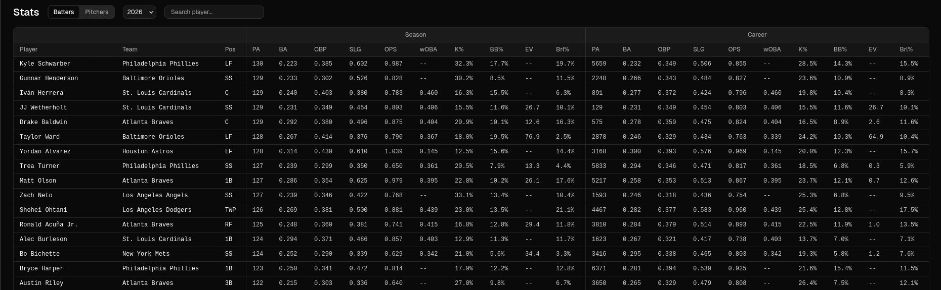
Two things follow from this. One, the sim and the dashboard read from the same source of truth, so a stats discrepancy is a data bug, not a model-versus-display mismatch. Two, the same DuckDB engine that runs my analytic queries also runs the model's feature lookups at inference time, with DuckLake managing transactions across both.

The model is a 22-class classifier over plate appearance outcomes: single, double, triple, home run, walk, hit-by-pitch, strikeout, ground-out, fly-out, and the rarer ones (sac fly, fielder's choice, GIDP, sac bunt, catcher interference). XGBoost on a vector of ~172 features per PA, with isotonic calibration applied on top of the raw probabilities.

The training is straightforward. The interesting decision was prioritizing calibration over accuracy. A 22-class model that picks the correct outcome 50% of the time is fine; one that says “30% chance of strikeout, 25% single, 15% walk” and is right about those frequencies in aggregate is far more useful downstream. The sim averages over thousands of simulated PAs per game; what matters is that the marginal distributions over outcomes are correct, not that any single PA's most-likely class lines up with the actual outcome.

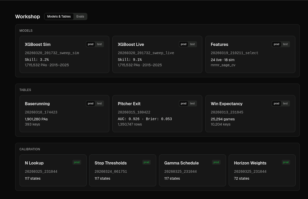
Everything above is a registered artifact. The model, the calibration table, the baserunning lookups, the WE table; each lives in the workshop view above with its own slot (prod, test, candidate, archived) and metrics. Promoting a new XGBoost run to prod is a single update, and the sim picks it up on the next inference. Eval results stay tied to the slot configuration that produced them, so when I look back at “the prod accuracy in March,” I know exactly which model + baserunning table + WE table produced it.

Turning a per-PA outcome model into a game-level win probability means projecting forward. Each plate appearance is a probabilistic step; the rest of the game is a tree of those steps. Monte Carlo just means sampling that tree: draw an outcome for the next PA, advance the state, repeat until the game ends. Do that many times and the fraction of paths where the home team wins is your win probability estimate.

Each path is a sample of how the rest of the game might play out. More paths, more information, tighter estimate. But each path is also expensive: sixty-some sequential model calls per simulated game. So the real question is information per compute. How long does each path need to be? How many paths do we need? And does either of those answers change with the situation?

How long does each path need to be?

The matchup edge decays with horizon. Past a few PAs the lineup turns over, the bullpen comes in, and whatever advantage the sim had over the WE table dissolves into noise. So instead of running paths to the end of the game, the estimator samples one half-inning forward, reads the WE table at the boundary, and treats that as the value of everything past the lookahead. The weights on those readings are calibrated per state via Markowitz minimum-variance over the WE-error covariance, with horizons gated to zero where the sim's Brier doesn't beat the entry baseline. About half the states find no horizon with an edge; for those the estimator returns WE directly without sampling.

How many paths do we need?

The variance of a Monte Carlo estimator shrinks as σ²/N (law of large numbers, 1/√N standard error). The wrinkle is that σ depends on the state we're starting from. A fixed N overspends on easy states (where p is near 0 or 1 and the variance is small) and underspends on hard ones (close games, where p is near 0.5 and σ is largest).

Two steps set the per-state count. First, an empirical convergence study: run the sim at N = 25, 50, 100, 200, 500 and watch the standard deviation of the estimate stop dropping. The smallest N at which it levels off is what the state actually needs. Second, a target-SE floor: from the standard sample-proportion formula sqrt(p(1-p)/N), pick the smallest N that gets SE ≤ 0.02 at the state's win-prob magnitude. The per-state path count is the max of the two.

High-leverage states get more paths. Decisive states get few. Same target precision across the board, compute spent where it actually buys it.

Can the paths run in parallel?

Yes. All paths for a given state advance one PA together as NumPy arrays, and the model fires a single batched ONNX call instead of one call per path. XGBoost batched inference ends up faster than per-row even when the micro-benchmarks look identical.

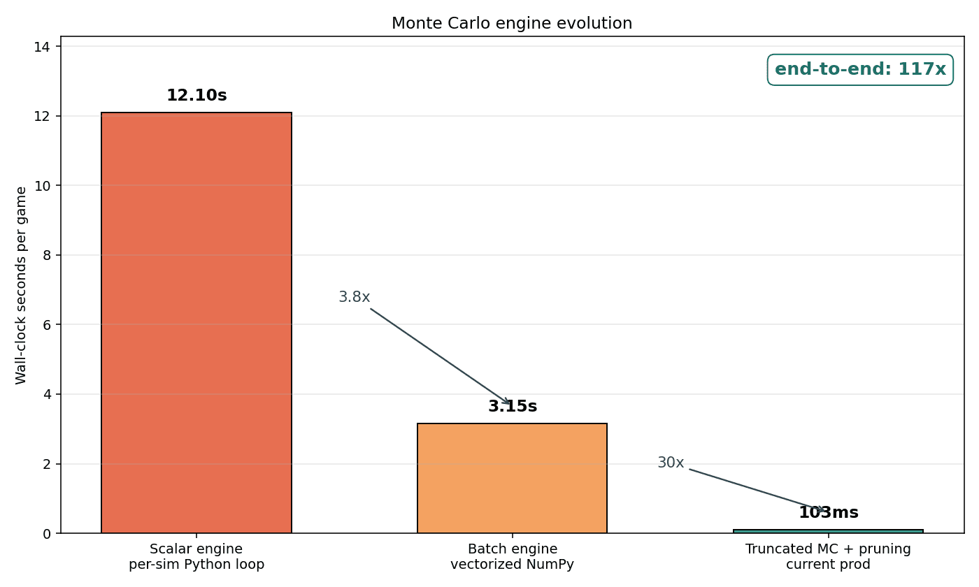
End to end, two orders of magnitude faster than the naive Python loop, with the compute concentrated on the states where matchup detail actually moves the answer.

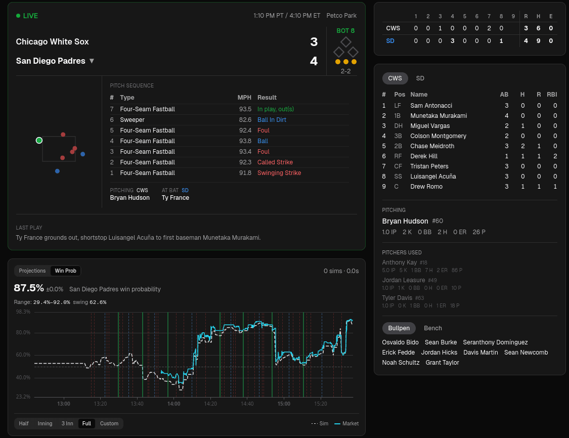
What comes out is a distribution: the dashboard shows the mean, the CI band from the sims, and the predicted swing range. None of that follows from a single WE-table number.

The tradeoff has been implicit since section 1. The WE table is a free lookup that already encodes a century of state-conditioned averages. The sim is matchup-aware compute that only buys something if its prediction is closer to truth than that lookup. The calibration step measures exactly that, per state bucket, on real outcomes. Its output is a per-state map of where the sim's prediction at each look-ahead beat WE.

Mechanically, the calibration step runs across every eval game in a given state bucket and asks, at each candidate look-ahead horizon, whether the sim's average squared error against actual outcomes is smaller than WE's error at the entry state. Horizons where the sim is closer to truth survive; horizons where it isn't get dropped.

The surviving horizons each give a noisy estimate of the same quantity but from different vantage points in the simulated game. Combining them isn't just averaging. Their errors are correlated because they share trajectories, so a naive mean would double-count overlapping information. The calibration computes the covariance matrix of those errors, applies Ledoit-Wolf shrinkage to keep it stable in buckets with few games, and inverts it. Plugged into the Markowitz minimum-variance formula w = Σ⁻¹·1 / (1ᵀ·Σ⁻¹·1), the result gives weights that downweight horizons whose noise is already absorbed by others and upweight horizons that contribute independent signal.

The output is a per-state weight vector that, paired with the surviving-horizon list, tells the sim how to combine its checkpoints into one prediction for that kind of state. Saved as an artifact, read by the runtime on every prediction.

Read across the 72 calibrated state buckets:

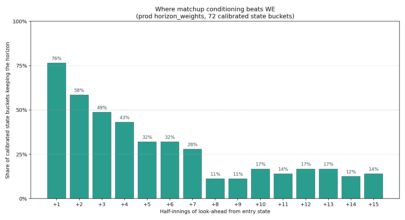
In 76% of buckets, the sim's one-half-inning lookahead beats WE. By four half-innings, only 43%. By eight, almost none.

The hypothesis: matchup signal lives in the next handful of plate appearances and gets averaged into noise after that. The lineup turns over, the bullpen comes in, and the round-bat-round-ball variance of subsequent play diffuses whatever edge a specific batter-pitcher matchup carries. By the time you're looking eight half-innings out, every comparable matchup that ever played from a similar state has averaged into WE's lookup, and there's nothing left for the sim to add.

The deeper reason the sim has to fight for ground: WE is calibrated by construction. Its predictions are the historical home-win frequencies from each state, so by definition they match observed outcomes in aggregate. The sim has to earn calibration through stochastic sampling, which costs variance from the PA model and from MC noise. Where matchup conditioning genuinely helps, that signal exceeds the variance overhead and the sim's prediction ends up tighter than WE's. Where it doesn't, the sim's noise budget costs more than the signal it gains. The Brier gate above is exactly this comparison; the buckets that survive are the ones where the matchup edge clears its own variance overhead.

That's the tradeoff the project navigates. Pay sim compute for the short window where matchup detail still moves the probability past what WE already encodes; take WE for free past that. The 49% runtime short-circuit is the same picture from a different angle: half the states the sim sees in production land in buckets where no horizon beat WE, so the runtime returns the table directly.

You don't really beat a lookup table that already encodes a century of how baseball plays out. You sit beside it for a stretch of plate appearances where the matchup is sharp enough to nudge the probability past the historical average, then the game absorbs whatever advantage was there and the table picks the rest up. What I came away with wasn't a verdict on the sim. It was respect for how much of baseball the WE table has already encoded, and how naturally the calibration ended up agreeing with it.